FRF and Prediction
Frequency response function estimation for one input or several, and the question that follows from it: given some channels, how much of another one can any linear model account for?
frf gives the H1/H2/H3 estimators with coherence alongside, because coherence
is what says whether either number is worth reading. frf_mimo solves the
several-inputs case and returns the condition number of the input spectral
matrix, which is the diagnostic that matters when inputs are correlated.
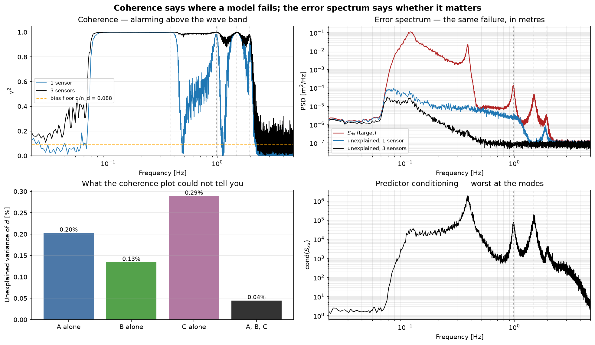
error_spectrum turns the same machinery around. Instead of asking what the
transfer function is, it asks what is left over: the residual spectrum of the
best linear predictor, in the target's own units. Report that rather than the
coherence alone — coherence says where a model fails, the error spectrum says
how much that matters, and the two often disagree.
dspkit.frf.frf(x, y, fs, estimator='H1', window='hann', nperseg=None, noverlap=None)
Frequency response function between one input and one output.
Parameters:
| Name | Type | Description | Default |
|---|---|---|---|
x
|
(array_like, shape(N))
|
Input (excitation), e.g. a measured force. |
required |
y
|
(array_like, shape(N))
|
Output (response), e.g. an acceleration. |
required |
fs
|
float
|
Sampling frequency [Hz]. |
required |
estimator
|
('H1', 'H2', 'H3')
|
Which estimator to form. See the notes. |
'H1'
|
window
|
str
|
Welch parameters, as elsewhere in the library. |
'hann'
|
nperseg
|
str
|
Welch parameters, as elsewhere in the library. |
'hann'
|
noverlap
|
str
|
Welch parameters, as elsewhere in the library. |
'hann'
|
Returns:
| Type | Description |
|---|---|
dict with keys
|
|
Notes
The three estimators differ only in which spectrum sits where, and they answer to different noise:
H1 = Gxy / Gxxassumes the noise is on the output. It is the usual default, and it is biased down at resonance, where the response is large and any input noise matters most.H2 = Gyy / Gyxassumes the noise is on the input. It is biased up at resonance and is the better choice at anti-resonances, where the output is small and output noise dominates.H3is their geometric mean, a compromise with no cleaner justification than that.
Coherence is returned alongside because it is what says whether either number is worth reading. Where coherence is near 1, H1 and H2 agree and the choice does not matter; where they disagree, coherence has already dropped and is telling you why.
Source code in dspkit/frf.py
dspkit.frf.frf_mimo(inputs, output, fs, window='hann', nperseg=None, noverlap=None, ridge=1e-10, min_segments=None)
Frequency response functions from several simultaneous inputs to one output.
Solves H = inv(Gxx) @ Gxy at each frequency, where Gxx is the
inputs' own cross-spectral matrix and Gxy the input-output
cross-spectrum. This is the multi-input generalisation of H1.
Parameters:
| Name | Type | Description | Default |
|---|---|---|---|
inputs
|
(array_like, shape(n_inputs, N))
|
Simultaneous excitations. |
required |
output
|
(array_like, shape(N))
|
The response. |
required |
fs
|
float
|
Sampling frequency [Hz]. |
required |
window
|
str
|
Welch parameters. |
'hann'
|
nperseg
|
str
|
Welch parameters. |
'hann'
|
noverlap
|
str
|
Welch parameters. |
'hann'
|
ridge
|
float
|
Regularisation added to the normalised input matrix before inversion. |
1e-10
|
min_segments
|
int or None
|
Refuse below this many Welch averages. Defaults to |
None
|
Returns:
| Type | Description |
|---|---|
dict with keys
|
|
Notes
Correlated inputs are the thing to watch, and coherence will not warn
you. If two shakers drive the structure in a correlated way, Gxx is
near-singular and the split of credit between the inputs is arbitrary --
the individual FRFs can be meaningless while together they still predict
the output perfectly. Measured on two inputs at 0.95 correlation, both the
multiple coherence (0.996) and the ordinary coherences (0.994, 0.993) stayed
high while the FRFs were not separable. Neither number tells you anything is
wrong.
input_condition is what does. It is the condition number of the
normalised input cross-spectral matrix: near 1 the inputs are distinguishable
and the FRFs mean something individually; large (say above 100) they are not,
and only their combined effect is identifiable. Drive the shakers with
uncorrelated signals if you need the FRFs separately.
Gxx is only invertible with more Welch averages than inputs. Below that
the result is arbitrary rather than merely noisy, so it is refused.
Source code in dspkit/frf.py
109 110 111 112 113 114 115 116 117 118 119 120 121 122 123 124 125 126 127 128 129 130 131 132 133 134 135 136 137 138 139 140 141 142 143 144 145 146 147 148 149 150 151 152 153 154 155 156 157 158 159 160 161 162 163 164 165 166 167 168 169 170 171 172 173 174 175 176 177 178 179 180 181 182 183 184 185 186 187 188 189 190 191 192 193 194 195 196 197 198 199 200 201 202 203 204 205 206 207 208 209 210 211 212 213 214 215 216 217 218 219 220 221 222 223 224 225 226 227 228 229 230 231 232 233 234 235 236 237 238 239 240 241 242 243 244 245 | |
dspkit.frf.error_spectrum(target, predictors, fs, window='hann', nperseg=None, noverlap=None, ridge=1e-10, min_segments=None)
How much of a signal the other channels cannot account for, per frequency.
Given a target d and one or more predictors x, the best linear
time-invariant model has a residual whose spectrum is fixed entirely by
the coherence::
S_ee(f) = [1 - gamma^2(f)] * S_dd(f)
with gamma^2 the ordinary coherence for one predictor and the multiple
coherence for several. The target spectrum splits into the part any linear
model driven by x can reproduce and the part none can::
S_dd = gamma^2 * S_dd  +  (1 - gamma^2) * S_dd
        coherent            error spectrum
This is the frequency-domain form of var_resid = (1 - r^2) var_y, with
gamma^2(f) playing the role of a frequency-local R-squared.
Parameters:
| Name | Type | Description | Default |
|---|---|---|---|
target
|
(array_like, shape(N))
|
The signal to be explained. |
required |
predictors
|
(array_like, shape(N) or (q, N))
|
The signals to explain it with. |
required |
fs
|
float
|
Sampling frequency [Hz]. |
required |
window
|
str
|
Welch parameters. |
'hann'
|
nperseg
|
str
|
Welch parameters. |
'hann'
|
noverlap
|
str
|
Welch parameters. |
'hann'
|
ridge
|
float
|
Regularisation of the normalised predictor matrix before inversion. |
1e-10
|
min_segments
|
int or None
|
Refuse below this many Welch averages. Defaults to |
None
|
Returns:
| Type | Description |
|---|---|
dict with keys
|
|
Notes
Report the error spectrum, not the coherence alone. Coherence is
dimensionless and says where a model fails; the error spectrum carries
the target's units and says how much that matters. A band where
gamma^2 collapses to zero is harmless if S_dd is negligible there,
and that is the usual case, because coherence is worst exactly where there
is no signal to be coherent about. Judging a model by the coherence plot
alone tends to produce needless alarm. Measured on the four-storey shear chain
in tests/test_frf_response.py, a single accelerometer averages a
coherence of 0.50 above the wave band, which looks like a broken model,
and still accounts for 99.8% of the target's variance -- because that
band carries two and a half decades less power than the wave band does.
Compare the coherence against bias_floor, not against zero. With
q predictors and n_d Welch averages, genuinely unrelated signals
give an expected coherence of about q / n_d. Adding predictors always
raises the apparent coherence, part of which is nothing but extra fitting
freedom, so the error spectrum returned here is biased downward --
optimistic. Models with different numbers of predictors cannot be ranked
on this number alone; hold out part of the record instead. A warning is
issued once the floor passes 0.1.
A too-short segment manufactures an error spectrum that is not there.
This is the failure mode to watch, and it is the opposite of the one
dspkit.spectral.coherence warns about. Let B_e be the resolution
bandwidth of the estimate (about 1.5 fs / nperseg for a Hann window)
and B_r = 2 zeta f_r the half-power bandwidth of the sharpest feature.
When B_e is not small next to B_r, leakage smears peaks and
notches, coherence is biased downward, and the spurious residual scales as
(B_e / B_r)^2. Keep B_e / B_r <= 1/4. Because the spurious part is
proportional to S_dd, it is worst where the target is strong, and it
can exceed the genuine residual. On a noise-free
single-input version of the same shear chain, where the true error
spectrum is exactly zero, the apparent unexplained variance runs
3.8e-5, 1.6e-4, 6.3e-4 and 2.4e-3 of the target as B_e / B_r goes
0.06, 0.12, 0.24, 0.49 -- a clean square law, and every bit of it an
artefact of the segment length.
Choose nperseg from the damping bandwidth of the sharpest mode and
then lengthen the record until the averages are adequate. Do not trade
resolution for averages when S_dd is large and sharply peaked.
What the residual contains cannot be separated here. Three distinct
mechanisms push gamma^2 below one and this decomposition sees only
their sum: measurement noise on either channel, inputs driving the system
that are not reflected in the predictors, and nonlinearity, which by
construction no H(f) can represent. Noise on a predictor is the
awkward one -- it inflates the denominator and biases the identified gain
towards zero, so the model is attenuated rather than merely noisy.
Telling the three apart needs more information: partial coherences,
repeated tests, or a physical model.
This is a lower bound for any causal predictor. The filters returned are the non-causal Wiener solution and use the whole record, past and future. A causal finite-order model is constrained by the Wiener-Hopf equations and cannot do better, so a fitted ARX or state-space predictor sitting well above this curve is limited by its model order, not by the physics.
See Also
frf_mimo, dspkit.multisensor.multiple_coherence, dspkit.multisensor.partial_coherence
Examples:
>>> import numpy as np
>>> from dspkit.frf import error_spectrum
>>> rng = np.random.default_rng(0)
>>> a = rng.normal(size=20000)
>>> d = np.convolve(a, np.ones(8) / 8, mode="same")
>>> r = error_spectrum(d, a, 100.0, nperseg=1024)
>>> bool(r["unexplained_fraction"] < 0.01)
True
Source code in dspkit/frf.py
248 249 250 251 252 253 254 255 256 257 258 259 260 261 262 263 264 265 266 267 268 269 270 271 272 273 274 275 276 277 278 279 280 281 282 283 284 285 286 287 288 289 290 291 292 293 294 295 296 297 298 299 300 301 302 303 304 305 306 307 308 309 310 311 312 313 314 315 316 317 318 319 320 321 322 323 324 325 326 327 328 329 330 331 332 333 334 335 336 337 338 339 340 341 342 343 344 345 346 347 348 349 350 351 352 353 354 355 356 357 358 359 360 361 362 363 364 365 366 367 368 369 370 371 372 373 374 375 376 377 378 379 380 381 382 383 384 385 386 387 388 389 390 391 392 393 394 395 396 397 398 399 400 401 402 403 404 405 406 407 408 409 410 411 412 413 414 415 416 417 418 419 420 421 422 423 424 425 426 427 428 429 430 431 432 433 434 435 436 437 438 | |