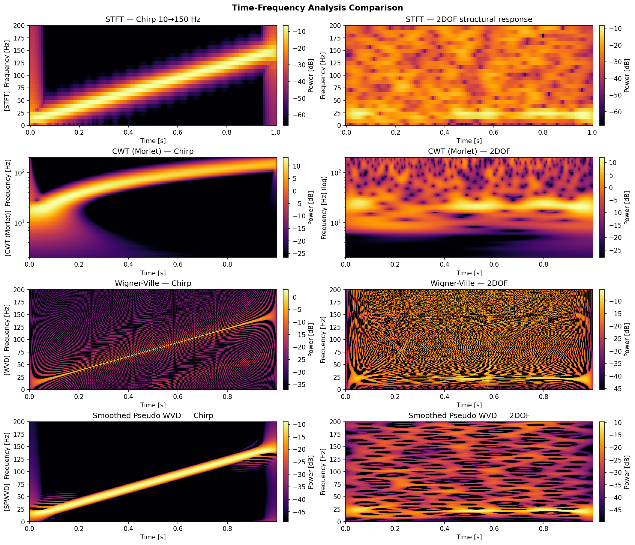
Skip to content

Time-Frequency

Joint time-frequency representations for non-stationary signals.

Function Resolution Cross-terms Cost
stft Window-limited None O(N log N)
cwt_scalogram Adaptive (log-freq) None O(N log N)
wigner_ville Optimal Yes O(N²)
smoothed_pseudo_wv Tunable Reduced O(N²)

WVD/SPWVD computation time

Both Wigner-Ville functions are O(N²). For signals longer than ~2048 samples a UserWarning is raised. Use warn_above to adjust the threshold.

Time-frequency analysis example


STFT

dspkit.timefreq.stft(x, fs, window='hann', nperseg=256, noverlap=None, scaling='spectrum')

Short-Time Fourier Transform.

Parameters:

Name Type Description Default
x (array_like, shape(N))
required
fs float

Sampling frequency [Hz].

required
window str

Window function (default 'hann').

'hann'
nperseg int

Segment length [samples]. Larger → better frequency resolution, worse time resolution. Default 256.

256
noverlap int or None

Overlapping samples between segments. Defaults to nperseg * 3 // 4 (75 %) for smooth output.

None
scaling (spectrum, psd)

'spectrum' normalises as amplitude; 'psd' as power density.

'spectrum'

Returns:

Name Type Description
freqs (ndarray, shape(nperseg // 2 + 1))

Frequency vector [Hz].

times ndarray

Time vector [s], centre of each segment.

Zxx (ndarray, shape(len(freqs), len(times)), complex)

STFT coefficients. np.abs(Zxx) is the spectrogram amplitude.

Source code in dspkit/timefreq.py
def stft(
    x: np.ndarray,
    fs: float,
    window: str = "hann",
    nperseg: int = 256,
    noverlap: int | None = None,
    scaling: Literal["spectrum", "psd"] = "spectrum",
) -> tuple[np.ndarray, np.ndarray, np.ndarray]:
    """
    Short-Time Fourier Transform.

    Parameters
    ----------
    x : array_like, shape (N,)
    fs : float
        Sampling frequency [Hz].
    window : str
        Window function (default ``'hann'``).
    nperseg : int
        Segment length [samples]. Larger → better frequency resolution,
        worse time resolution. Default 256.
    noverlap : int or None
        Overlapping samples between segments. Defaults to
        ``nperseg * 3 // 4`` (75 %) for smooth output.
    scaling : {'spectrum', 'psd'}
        ``'spectrum'`` normalises as amplitude; ``'psd'`` as power density.

    Returns
    -------
    freqs : ndarray, shape (nperseg // 2 + 1,)
        Frequency vector [Hz].
    times : ndarray
        Time vector [s], centre of each segment.
    Zxx : ndarray, shape (len(freqs), len(times)), complex
        STFT coefficients. ``np.abs(Zxx)`` is the spectrogram amplitude.
    """
    x = np.asarray(x, dtype=float)
    if noverlap is None:
        noverlap = nperseg * 3 // 4
    freqs, times, Zxx = _signal.stft(
        x, fs=fs, window=window, nperseg=nperseg, noverlap=noverlap, scaling=scaling
    )
    return freqs, times, Zxx

CWT Scalogram

dspkit.timefreq.cwt_scalogram(x, fs, freqs=None, w=6.0)

Continuous Wavelet Transform scalogram using the complex Morlet wavelet.

The Morlet wavelet provides excellent time-frequency localisation for oscillatory signals and is standard in structural dynamics.

The parameter w sets the number of oscillations in the wavelet (its centre frequency in rad):

  • Higher w → better frequency resolution, worse time resolution.
  • Lower w → better time resolution, worse frequency resolution.

Parameters:

Name Type Description Default
x (array_like, shape(N))
required
fs float

Sampling frequency [Hz].

required
freqs array_like or None

Analysis frequencies [Hz]. Defaults to 50 log-spaced values from 1 Hz to fs / 4.

None
w float

Morlet centre-frequency parameter (default 6.0).

6.0

Returns:

Name Type Description
freqs ndarray

Analysis frequencies [Hz].

times (ndarray, shape(N))

Time vector [s].

W (ndarray, shape(len(freqs), N), complex)

CWT coefficients. np.abs(W) is the scalogram amplitude; np.abs(W) ** 2 is the energy density.

Source code in dspkit/timefreq.py
def cwt_scalogram(
    x: np.ndarray,
    fs: float,
    freqs: np.ndarray | None = None,
    w: float = 6.0,
) -> tuple[np.ndarray, np.ndarray, np.ndarray]:
    """
    Continuous Wavelet Transform scalogram using the complex Morlet wavelet.

    The Morlet wavelet provides excellent time-frequency localisation
    for oscillatory signals and is standard in structural dynamics.

    The parameter ``w`` sets the number of oscillations in the wavelet
    (its centre frequency in rad):

    - Higher ``w`` → better frequency resolution, worse time resolution.
    - Lower  ``w`` → better time resolution, worse frequency resolution.

    Parameters
    ----------
    x : array_like, shape (N,)
    fs : float
        Sampling frequency [Hz].
    freqs : array_like or None
        Analysis frequencies [Hz]. Defaults to 50 log-spaced values from
        1 Hz to ``fs / 4``.
    w : float
        Morlet centre-frequency parameter (default 6.0).

    Returns
    -------
    freqs : ndarray
        Analysis frequencies [Hz].
    times : ndarray, shape (N,)
        Time vector [s].
    W : ndarray, shape (len(freqs), N), complex
        CWT coefficients. ``np.abs(W)`` is the scalogram amplitude;
        ``np.abs(W) ** 2`` is the energy density.
    """
    x = np.asarray(x, dtype=float)
    N = len(x)
    if freqs is None:
        freqs = np.geomspace(1.0, fs / 4.0, num=50)
    else:
        freqs = np.asarray(freqs, dtype=float)

    # Scale-to-frequency: f = w * fs / (2π * a) → a = w * fs / (2π * f)
    scales = w * fs / (2.0 * np.pi * freqs)

    # FFT-based CWT — no external wavelet library required.
    #
    # The analytic complex Morlet wavelet:
    #   ψ(t) = π^(-1/4) * exp(j*w*t) * exp(-t²/2)
    # Its Fourier transform (one-sided, analytic):
    #   Ψ(ω) = π^(-1/4) * sqrt(2π) * exp(-(ω-w)²/2)  for ω > 0,  0 otherwise
    # Scaled version (scale = a):
    #   Ψ_a(ω) = π^(-1/4) * sqrt(2π·a) * exp(-(a·ω - w)²/2)
    #
    # CWT via Fourier convolution theorem:
    #   W(a, b) = IFFT{ X(ω) · Ψ_a*(ω) }
    # Since Ψ_a is real (Gaussian), Ψ_a* = Ψ_a.
    #
    # Zero-padding to 2N reduces circular convolution wrap-around at edges.
    Nfft = 2 * N
    X = np.fft.fft(x, n=Nfft)
    xi = 2.0 * np.pi * np.fft.fftfreq(Nfft)  # angular frequency [rad/sample]

    W = np.zeros((len(scales), N), dtype=complex)
    c = np.pi ** -0.25  # normalisation constant

    for i, a in enumerate(scales):
        psi_hat = np.where(
            xi > 0,
            c * np.sqrt(2.0 * np.pi * a) * np.exp(-0.5 * (a * xi - w) ** 2),
            0.0,
        )
        W[i, :] = np.fft.ifft(X * psi_hat)[:N]

    times = np.arange(N) / fs
    return freqs, times, W

Wigner-Ville Distribution

dspkit.timefreq.wigner_ville(x, fs, warn_above=2048)

Wigner-Ville Distribution (WVD).

Computed via the analytic signal (Hilbert transform) to suppress aliasing artifacts. The result is real-valued.

The WVD achieves the highest joint time-frequency resolution of any bilinear distribution and satisfies both the time and frequency marginals exactly for single-component signals. However, it produces oscillatory cross-terms between signal components. For noisy or multi-component signals, prefer smoothed_pseudo_wv.

.. warning:: Computation is O(N²) in time and memory.

Parameters:

Name Type Description Default
x (array_like, shape(N))
required
fs float

Sampling frequency [Hz].

required
warn_above int

Emit a warning when len(x) exceeds this value (default 2048).

2048

Returns:

Name Type Description
freqs (ndarray, shape(N // 2 + 1))

Frequency vector [Hz], from 0 to fs / 4. The half-lag autocorrelation limits the representable frequency range to fs/4 (Nyquist of the half-lag domain).

times (ndarray, shape(N))

Time vector [s].

WVD (ndarray, shape(N, N // 2 + 1))

Wigner-Ville distribution. May contain negative values (cross-terms or edge effects). Integrating over frequency yields instantaneous power.

Source code in dspkit/timefreq.py
def wigner_ville(
    x: np.ndarray,
    fs: float,
    warn_above: int = 2048,
) -> tuple[np.ndarray, np.ndarray, np.ndarray]:
    """
    Wigner-Ville Distribution (WVD).

    Computed via the analytic signal (Hilbert transform) to suppress
    aliasing artifacts. The result is real-valued.

    The WVD achieves the highest joint time-frequency resolution of any
    bilinear distribution and satisfies both the time and frequency
    marginals exactly for single-component signals. However, it produces
    oscillatory cross-terms between signal components. For noisy or
    multi-component signals, prefer ``smoothed_pseudo_wv``.

    .. warning::
        Computation is O(N²) in time and memory.

    Parameters
    ----------
    x : array_like, shape (N,)
    fs : float
        Sampling frequency [Hz].
    warn_above : int
        Emit a warning when ``len(x)`` exceeds this value (default 2048).

    Returns
    -------
    freqs : ndarray, shape (N // 2 + 1,)
        Frequency vector [Hz], from 0 to fs / 4.
        The half-lag autocorrelation limits the representable frequency
        range to fs/4 (Nyquist of the half-lag domain).
    times : ndarray, shape (N,)
        Time vector [s].
    WVD : ndarray, shape (N, N // 2 + 1)
        Wigner-Ville distribution. May contain negative values (cross-terms
        or edge effects). Integrating over frequency yields instantaneous power.
    """
    x = np.asarray(x, dtype=float)
    N = len(x)

    if N > warn_above:
        warnings.warn(
            f"wigner_ville: N={N} > {warn_above}. WVD is O(N²) — "
            "consider decimating or passing a shorter segment.",
            stacklevel=2,
        )

    z = _signal.hilbert(x)  # analytic signal

    # Build instantaneous autocorrelation R[n, m] = z[n+m] * conj(z[n-m])
    # stored as an N×N complex matrix using circular (Hermitian) indexing:
    #   column 0            → half-lag m=0
    #   columns 1..N//2     → positive half-lags
    #   columns N//2+1..N-1 → negative half-lags (conjugate of positive)
    #
    # Because R[n,m] = A²·exp(j·4π·f₀·m/fs) for a pure tone at f₀,
    # the N-point DFT peaks at bin k = 2·N·f₀/fs.  The correct frequency
    # mapping is therefore  f_k = k·fs/(2N), i.e. rfftfreq(N, d=2/fs).
    # This covers 0 to fs/4 (the Nyquist limit of the half-lag domain).
    # Dividing by fs normalises the power marginal:
    #   ∑_k W[n, k] · Δf  ≈  A²/2   (RMS power of a real sine of amplitude A).
    R = np.zeros((N, N), dtype=complex)
    R[:, 0] = np.abs(z) ** 2  # m=0

    for m in range(1, N // 2 + 1):
        ns = np.arange(m, N - m)  # valid time indices for this lag
        if len(ns) == 0:
            continue
        vals = z[ns + m] * np.conj(z[ns - m])
        R[ns, m] = vals
        R[ns, N - m] = np.conj(vals)  # Hermitian symmetry → real output

    WVD_full = 2.0 * np.real(np.fft.fft(R, axis=1)) / fs
    freqs = np.fft.rfftfreq(N, d=2.0 / fs)   # 0 … fs/4, length N//2+1
    times = np.arange(N) / fs
    return freqs, times, WVD_full[:, : len(freqs)]

Smoothed Pseudo WVD

dspkit.timefreq.smoothed_pseudo_wv(x, fs, lag_samples=None, time_samples=None, warn_above=2048)

Smoothed Pseudo Wigner-Ville Distribution (SPWVD).

Suppresses the cross-term interference of the plain WVD by applying:

  • A Hann lag window of half-length lag_samples: limits the autocorrelation lag, smoothing the frequency axis and attenuating cross-terms between components at different frequencies.
  • A Hann time window of half-length time_samples: smooths the time axis and attenuates cross-terms between components at different times.

Increasing either window suppresses more cross-terms but reduces the corresponding resolution. Choose window sizes smaller than the signal's characteristic time/frequency separation.

.. warning:: Computation is O(N²) in time and memory.

Parameters:

Name Type Description Default
x (array_like, shape(N))
required
fs float

Sampling frequency [Hz].

required
lag_samples int or None

Half-length of the Hann lag window [samples]. Full window = 2 * lag_samples + 1. Defaults to max(N // 8, 4).

None
time_samples int or None

Half-length of the Hann time window [samples]. Defaults to max(N // 8, 4).

None
warn_above int

Emit a warning when len(x) exceeds this value (default 2048).

2048

Returns:

Name Type Description
freqs (ndarray, shape(N // 2 + 1))

Frequency vector [Hz], from 0 to fs / 4.

times (ndarray, shape(N))

Time vector [s].

SPWVD (ndarray, shape(N, N // 2 + 1))

Smoothed distribution. Tends to non-negative after sufficient smoothing.

Source code in dspkit/timefreq.py
def smoothed_pseudo_wv(
    x: np.ndarray,
    fs: float,
    lag_samples: int | None = None,
    time_samples: int | None = None,
    warn_above: int = 2048,
) -> tuple[np.ndarray, np.ndarray, np.ndarray]:
    """
    Smoothed Pseudo Wigner-Ville Distribution (SPWVD).

    Suppresses the cross-term interference of the plain WVD by applying:

    - A **Hann lag window** of half-length ``lag_samples``: limits the
      autocorrelation lag, smoothing the frequency axis and attenuating
      cross-terms between components at different frequencies.
    - A **Hann time window** of half-length ``time_samples``: smooths the
      time axis and attenuates cross-terms between components at different
      times.

    Increasing either window suppresses more cross-terms but reduces the
    corresponding resolution. Choose window sizes smaller than the signal's
    characteristic time/frequency separation.

    .. warning::
        Computation is O(N²) in time and memory.

    Parameters
    ----------
    x : array_like, shape (N,)
    fs : float
        Sampling frequency [Hz].
    lag_samples : int or None
        Half-length of the Hann lag window [samples].
        Full window = ``2 * lag_samples + 1``. Defaults to ``max(N // 8, 4)``.
    time_samples : int or None
        Half-length of the Hann time window [samples].
        Defaults to ``max(N // 8, 4)``.
    warn_above : int
        Emit a warning when ``len(x)`` exceeds this value (default 2048).

    Returns
    -------
    freqs : ndarray, shape (N // 2 + 1,)
        Frequency vector [Hz], from 0 to fs / 4.
    times : ndarray, shape (N,)
        Time vector [s].
    SPWVD : ndarray, shape (N, N // 2 + 1)
        Smoothed distribution. Tends to non-negative after sufficient smoothing.
    """
    x = np.asarray(x, dtype=float)
    N = len(x)

    if N > warn_above:
        warnings.warn(
            f"smoothed_pseudo_wv: N={N} > {warn_above}. SPWVD is O(N²) — "
            "consider decimating or passing a shorter segment.",
            stacklevel=2,
        )

    if lag_samples is None:
        lag_samples = max(N // 8, 4)
    if time_samples is None:
        time_samples = max(N // 8, 4)

    z = _signal.hilbert(x)

    # Lag (frequency) window: Hann of length 2*L+1
    L = lag_samples
    lag_win = _signal.windows.hann(2 * L + 1)  # lag_win[L + m] = weight at lag m

    R = np.zeros((N, N), dtype=complex)
    R[:, 0] = np.abs(z) ** 2 * lag_win[L]  # m=0

    for m in range(1, min(L + 1, N // 2 + 1)):
        g_m = lag_win[L + m]
        if g_m == 0.0:
            continue
        ns = np.arange(m, N - m)
        if len(ns) == 0:
            continue
        vals = g_m * z[ns + m] * np.conj(z[ns - m])
        R[ns, m] = vals
        R[ns, N - m] = np.conj(vals)

    # Time smoothing via Hann window convolved along axis 0 (time).
    h = _signal.windows.hann(2 * time_samples + 1)
    h = h / h.sum()
    R_real = _ndimage.convolve1d(R.real, h, axis=0, mode="constant", cval=0.0)
    R_imag = _ndimage.convolve1d(R.imag, h, axis=0, mode="constant", cval=0.0)
    R = R_real + 1j * R_imag

    SPWVD_full = 2.0 * np.real(np.fft.fft(R, axis=1)) / fs
    freqs = np.fft.rfftfreq(N, d=2.0 / fs)   # 0 … fs/4, length N//2+1
    times = np.arange(N) / fs
    return freqs, times, SPWVD_full[:, : len(freqs)]