Statistics
Probability density estimation and joint statistics for signal characterisation: KDE, histograms, joint distributions, covariance, Mahalanobis distance, normality assessment, and mutual information for dependence that coherence cannot see.
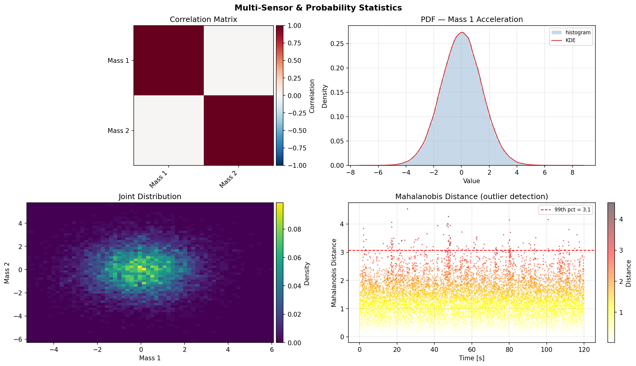
dspkit.statistics.pdf_estimate(x, n_points=256, bandwidth=None)
Kernel density estimate (KDE) of a signal's probability density function.
Uses a Gaussian kernel with automatic or user-specified bandwidth.
Parameters:
| Name | Type | Description | Default |
|---|---|---|---|
x
|
(array_like, shape(N))
|
Signal samples. |
required |
n_points
|
int
|
Number of evaluation points (default 256). |
256
|
bandwidth
|
float or None
|
KDE bandwidth (standard deviation of the Gaussian kernel).
If |
None
|
Returns:
| Name | Type | Description |
|---|---|---|
xi |
(ndarray, shape(n_points))
|
Evaluation points (range of |
density |
(ndarray, shape(n_points))
|
Estimated PDF values. |
Source code in dspkit/statistics.py
dspkit.statistics.histogram(x, bins=50, density=True)
Normalised histogram (empirical PDF approximation).
Parameters:
| Name | Type | Description | Default |
|---|---|---|---|
x
|
(array_like, shape(N))
|
Signal samples. |
required |
bins
|
int or array_like
|
Number of bins or bin edges. |
50
|
density
|
bool
|
If |
True
|
Returns:
| Name | Type | Description |
|---|---|---|
bin_centres |
ndarray
|
Centre of each bin. |
counts |
ndarray
|
Histogram values (probability density if |
Source code in dspkit/statistics.py
dspkit.statistics.joint_histogram(x, y, bins=50, density=True)
2D histogram (empirical joint PDF) of two signals.
Parameters:
| Name | Type | Description | Default |
|---|---|---|---|
x
|
(array_like, shape(N))
|
Signal samples (must have equal length). |
required |
y
|
(array_like, shape(N))
|
Signal samples (must have equal length). |
required |
bins
|
int or (int, int)
|
Number of bins in each dimension. |
50
|
density
|
bool
|
If |
True
|
Returns:
| Name | Type | Description |
|---|---|---|
x_centres |
(ndarray, shape(nx))
|
Bin centres along x. |
y_centres |
(ndarray, shape(ny))
|
Bin centres along y. |
H |
(ndarray, shape(nx, ny))
|
Joint histogram values. |
Source code in dspkit/statistics.py
dspkit.statistics.covariance_matrix(data, bias=False)
Covariance matrix for multi-channel data.
Parameters:
| Name | Type | Description | Default |
|---|---|---|---|
data
|
(array_like, shape(n_channels, N))
|
Each row is a time series from one sensor. |
required |
bias
|
bool
|
If |
False
|
Returns:
| Name | Type | Description |
|---|---|---|
C |
(ndarray, shape(n_channels, n_channels))
|
Covariance matrix. |
Source code in dspkit/statistics.py
dspkit.statistics.mahalanobis(data, reference=None)
Mahalanobis distance of each time sample from the distribution centre.
Useful for multivariate outlier detection in multi-channel SHM data.
D_M(x) = sqrt( (x - μ)^T · Σ^{-1} · (x - μ) )
Parameters:
| Name | Type | Description | Default |
|---|---|---|---|
data
|
(array_like, shape(n_channels, N))
|
Multi-channel time series. Each column is one observation. |
required |
reference
|
(array_like, shape(n_channels, N_ref) or None)
|
Reference data to compute the mean and covariance from.
If |
None
|
Returns:
| Name | Type | Description |
|---|---|---|
distances |
(ndarray, shape(N))
|
Mahalanobis distance of each time sample. |
Source code in dspkit/statistics.py
dspkit.statistics.qq_normal(x, line='ols')
Data for a normal Q-Q plot: theoretical quantiles, sample quantiles, line.
Returns the numbers, not a plot, in keeping with the rest of the library —
dspkit.plots wraps it for drawing. Plotting ordered against
theoretical gives a straight line if the sample is normal; curvature
at the ends is a tail departure, an S-shape is skew.
Parameters:
| Name | Type | Description | Default |
|---|---|---|---|
x
|
(array_like, shape(N))
|
Signal samples. Non-finite values are dropped. |
required |
line
|
(ols, quartile)
|
How the reference line is fitted.
|
'ols'
|
Returns:
| Name | Type | Description |
|---|---|---|
theoretical |
(ndarray, shape(N))
|
Standard-normal quantiles at the plotting positions, ascending. |
ordered |
(ndarray, shape(N))
|
The sample sorted ascending — the matching empirical quantiles. |
slope |
float
|
Slope of the reference line. For a normal sample it estimates the standard deviation. |
intercept |
float
|
Intercept of the reference line. For a normal sample it estimates the mean. |
Notes
Plotting positions are (k - a) / (N + 1 - 2a) with a = 3/8 for
N <= 10 and a = 1/2 above, the same convention scipy uses.
The reference line is not neutral, and this is the thing to know before
reading a Q-Q plot as evidence. A least-squares line is fitted to all N
points, and the extreme order statistics are the most spread out along the
x-axis, so they carry the most leverage: heavy tails tilt the line towards
themselves and thereby hide part of their own departure. 'quartile'
fits the bulk and lets the tails fall where they fall, which is what you
want when the tails are the question. Neither line is a fit "to the
normal distribution" — both are fitted to the data.
What this will not tell you: whether a departure is large enough to
matter, or whether it is real rather than sampling scatter. Q-Q plots of
normal samples wander visibly at the ends even at large N, because the
variance of an extreme order statistic is large. Read it alongside
normality, which puts numbers on the same departures.
See Also
normality
Examples:
>>> import numpy as np
>>> from dspkit.statistics import qq_normal
>>> x = np.random.default_rng(0).normal(2.0, 3.0, 5000)
>>> t, o, slope, intercept = qq_normal(x)
>>> bool(abs(slope - 3.0) < 0.2), bool(abs(intercept - 2.0) < 0.2)
(True, True)
Source code in dspkit/statistics.py
218 219 220 221 222 223 224 225 226 227 228 229 230 231 232 233 234 235 236 237 238 239 240 241 242 243 244 245 246 247 248 249 250 251 252 253 254 255 256 257 258 259 260 261 262 263 264 265 266 267 268 269 270 271 272 273 274 275 276 277 278 279 280 281 282 283 284 285 286 287 288 289 290 291 292 293 294 295 296 297 298 299 300 301 302 303 304 305 306 307 308 309 310 | |
dspkit.statistics.normality(x, shapiro_max_n=5000, large_n=5000, seed=0)
Normality indicators with the guidance needed to read them.
Returns effect sizes (skewness, excess kurtosis) and the four standard tests — D'Agostino K², Jarque-Bera, Anderson-Darling, Shapiro-Wilk — each with a plain-language interpretation and an explicit statement of whether it can be trusted at this sample size.
Parameters:
| Name | Type | Description | Default |
|---|---|---|---|
x
|
(array_like, shape(N))
|
Signal samples. Non-finite values are dropped. |
required |
shapiro_max_n
|
int
|
Shapiro-Wilk is computed on a random subsample of at most this many points (default 5000); above it the test's own approximation degrades. Pass 0 to skip Shapiro-Wilk entirely. |
5000
|
large_n
|
int
|
Sample size above which p-values are reported as uninformative (default 5000). See Notes. |
5000
|
seed
|
int or None
|
Seed for the Shapiro-Wilk subsample. Defaults to 0 so that repeated
calls on the same record agree; pass |
0
|
Returns:
| Name | Type | Description |
|---|---|---|
result |
dict
|
Anderson-Darling reports |
Notes
At a realistic record length every one of these tests rejects, and that
is a property of the test, not of the signal. A normality test asks "is
the departure larger than sampling scatter?", and sampling scatter shrinks
as 1/sqrt(N). With 20 000 samples a skew of 0.03 — visually and physically
nothing — is detected with certainty, so p < 1e-16 is the expected result
for real data and carries no information about how non-Gaussian the signal
is. Above large_n every test is therefore marked
reliable=False, and the effect sizes are what remain worth reading:
they are estimates of a fixed property of the distribution, and they get
better, not more damning, as N grows.
The tests also assume independent samples, which a vibration record is not. Serial correlation reduces the effective sample size, so the true scatter is wider than any of these p-values or the reported standard errors assume. The direction of that error is towards over-rejection, on top of the large-N effect above.
Shapiro-Wilk is the most powerful of the four at small N and the
least usable at large N: its approximation is documented as unreliable
much beyond 5000 samples. Rather than skip it or report a number known to
be wrong, it is computed on a random subsample of shapiro_max_n
points, and 'subsampled' and 'n_used' say so. Subsampling costs
power and does not repair the independence assumption.
What this will not tell you: whether the signal is stationary (a record
that switches between two Gaussian regimes is non-Gaussian overall while
every part of it is Gaussian), whether non-normality means damage, or
which samples caused it. For a signal that is Gaussian in the bulk and
not in the tails, qq_normal shows where the departure sits, which no
scalar here does.
See Also
qq_normal, dspkit.indicators.kurtosis, dspkit.indicators.skewness
Examples:
>>> import numpy as np
>>> from dspkit.statistics import normality
>>> x = np.random.default_rng(0).standard_t(df=4, size=4000)
>>> r = normality(x)
>>> r['n']
4000
>>> bool(r['excess_kurtosis']['value'] > 1.0)     # t(4) has heavy tails
True
Source code in dspkit/statistics.py
379 380 381 382 383 384 385 386 387 388 389 390 391 392 393 394 395 396 397 398 399 400 401 402 403 404 405 406 407 408 409 410 411 412 413 414 415 416 417 418 419 420 421 422 423 424 425 426 427 428 429 430 431 432 433 434 435 436 437 438 439 440 441 442 443 444 445 446 447 448 449 450 451 452 453 454 455 456 457 458 459 460 461 462 463 464 465 466 467 468 469 470 471 472 473 474 475 476 477 478 479 480 481 482 483 484 485 486 487 488 489 490 491 492 493 494 495 496 497 498 499 500 501 502 503 504 505 506 507 508 509 510 511 512 513 514 515 516 517 518 519 520 521 522 523 524 525 526 527 528 529 530 531 532 533 534 535 536 537 538 539 540 541 542 543 544 545 546 547 548 549 550 551 552 553 554 555 556 557 558 559 560 561 562 563 564 565 566 567 568 569 570 571 572 573 574 575 576 577 578 579 580 581 582 583 584 585 586 587 588 589 590 591 592 593 594 595 596 597 598 599 600 601 602 603 604 605 606 607 608 609 610 611 612 613 614 615 616 617 618 619 620 621 622 623 624 625 626 627 628 629 630 631 632 633 634 635 636 637 638 639 640 641 642 643 644 645 646 647 648 649 650 651 652 653 654 655 656 657 658 659 660 661 662 663 664 665 666 667 668 669 670 671 672 673 674 675 676 677 678 679 680 681 682 683 684 685 686 687 688 689 | |
dspkit.statistics.mutual_information(x, y, k=3, lags=0, standardize=True, jitter=True, seed=0)
Mutual information between two signals, by k-nearest-neighbour estimation.
I(X;Y) in nats — the dependence between two channels of any shape, not only the linear, same-frequency dependence coherence measures. It is zero if and only if the two are independent, which makes it the right tool for a relationship that is nonlinear (a rectifying joint, a rattle that responds to amplitude rather than to phase) or that lives at a lag.
Uses the Kraskov-Stogbauer-Grassberger estimator (algorithm 1): binned estimators are badly biased at realistic sample sizes because the answer depends on a bin width nobody can choose defensibly.
Parameters:
| Name | Type | Description | Default |
|---|---|---|---|
x
|
(array_like, shape(N))
|
The two signals, equal length. |
required |
y
|
(array_like, shape(N))
|
The two signals, equal length. |
required |
k
|
int
|
Number of nearest neighbours (default 3). Small k means low bias and high variance; k = 3 or 4 is the usual compromise. |
3
|
lags
|
int or array_like
|
Lag(s) in samples. MI is computed between |
0
|
standardize
|
bool
|
Scale each signal to unit variance first (default True). MI is invariant to this in theory; the estimator is not, because its neighbourhoods are squares in the joint (x, y) plane, so without it the answer depends on the relative units of the two channels. |
True
|
jitter
|
bool
|
Add noise at 1e-10 of the signal spread to break exact ties (default True). Quantised or clipped signals otherwise produce degenerate neighbour counts. |
True
|
seed
|
int or None
|
Seed for the jitter, so repeated calls agree. |
0
|
Returns:
| Name | Type | Description |
|---|---|---|
mi |
float or ndarray
|
Mutual information in nats — a float if |
Notes
Lags. MI has no frequency decomposition, so a lagged relationship is
invisible unless you look for it: at lag 0 a pure delay of half a period
can read as independence. Pass a range of lags and read the curve.
Every lag in a scan is estimated from the same number of samples — the
window is shrunk once, by the full span of the requested lags — because
the estimator's bias depends on N, and a curve whose sample count varies
along it is not comparable with itself.
Two things the lag scan does not fix. The maximum over a scan of L lags
is a biased estimate of the maximum: scanning inflates it, and the
inflation grows with L, so max(mi) from a wide scan is not comparable
with a single-lag value. And a lag scan finds a fixed delay; a
relationship spread over many lags (any filtered path) shows up weakly at
each one.
Significance. The number this returns is not a verdict, and it has no
natural scale to compare against: unlike coherence there is no [0, 1]
range and no fixed value that means "independent". The estimate for truly
independent signals is a small positive number that depends on N and k,
so "MI = 0.02 nats" is meaningless on its own. Establishing whether a
value is more than that floor requires a null distribution built from the
same data — use mi_significance, which does it with time-shifted
surrogates. A bare MI value with no surrogate test establishes
nothing.
What this will not tell you: direction or causality (MI is symmetric —
I(X;Y) = I(Y;X), and a lag peak is evidence of order, not of cause),
which frequency the dependence lives at, or the shape of the
relationship. It is also O(N log N) per lag with a KD-tree, so a wide
scan on a long record is seconds, not milliseconds.
See Also
mi_significance, dspkit.multisensor.partial_coherence, dspkit.spectral.coherence
Examples:
>>> import numpy as np
>>> from dspkit.statistics import mutual_information
>>> rng = np.random.default_rng(0)
>>> x = rng.normal(size=4000)
>>> quad = x ** 2 + 0.1 * rng.normal(size=4000)   # zero correlation
>>> bool(abs(np.corrcoef(x, quad)[0, 1]) < 0.05)
True
>>> bool(mutual_information(x, quad) > 0.3)       # but not independent
True
Source code in dspkit/statistics.py
777 778 779 780 781 782 783 784 785 786 787 788 789 790 791 792 793 794 795 796 797 798 799 800 801 802 803 804 805 806 807 808 809 810 811 812 813 814 815 816 817 818 819 820 821 822 823 824 825 826 827 828 829 830 831 832 833 834 835 836 837 838 839 840 841 842 843 844 845 846 847 848 849 850 851 852 853 854 855 856 857 858 859 860 861 862 863 864 865 866 867 868 869 870 871 872 873 874 875 876 877 878 879 880 881 882 883 884 885 886 887 888 889 890 891 892 | |
dspkit.statistics.mi_significance(x, y, k=3, lags=0, n_surrogates=199, method='shift', standardize=True, jitter=True, seed=0)
Is a mutual-information value more than the estimator's own floor?
Builds a null distribution by recomputing MI between x and surrogate
versions of y that carry no relationship to x, and reports where
the observed value falls in it. This is what turns an MI number into a
statement; without it, mutual_information returns a quantity with no
reference point.
Parameters:
| Name | Type | Description | Default |
|---|---|---|---|
x
|
(array_like, shape(N))
|
The two signals, equal length. |
required |
y
|
(array_like, shape(N))
|
The two signals, equal length. |
required |
k
|
int
|
Neighbours for the KSG estimator (default 3). |
3
|
lags
|
int or array_like
|
Lag or lags in samples, as in |
0
|
n_surrogates
|
int
|
Number of surrogates (default 199, giving a smallest attainable
p-value of 1/200 = 0.005). Cost is |
199
|
method
|
(shift, permutation)
|
How the surrogates are built. See Notes — the default matters. |
'shift'
|
standardize
|
bool
|
As in |
True
|
jitter
|
bool
|
As in |
True
|
seed
|
bool
|
As in |
True
|
Returns:
| Name | Type | Description |
|---|---|---|
result |
dict
|
|
Notes
Time-shifted surrogates are the default, and permutation is not. Permuting y destroys its autocorrelation as well as its relationship to x, so the null it builds is the null for "y is white noise", not for "y is unrelated to x". Real signals are strongly autocorrelated, the KSG floor rises with autocorrelation, and testing against a white-noise null therefore declares dependence far too readily. A circular time shift keeps each signal's own spectrum, distribution and autocorrelation exactly, and only destroys the alignment between them, which is the one thing under test. Shifts are drawn to exceed the widest requested lag, so a surrogate cannot accidentally re-align the pair.
method='permutation' is available for the case where the samples
genuinely are independent draws rather than a time series. Do not use it
on a vibration record.
p = (1 + #{null >= observed}) / (1 + n_surrogates), the standard
Monte-Carlo p-value, which cannot return 0: with 199 surrogates the
smallest value it can report is 0.005, and that means "not exceeded",
not "certain".
What this will not tell you: it tests one null — that the two signals are unrelated given each one's own autocorrelation. Rejecting it does not identify the shape of the relationship, its direction, or whether a third channel drives both. A shared excitation makes every sensor pair dependent, and this will report exactly that, correctly and uninformatively.
See Also
mutual_information
Examples:
>>> import numpy as np
>>> from dspkit.statistics import mi_significance
>>> rng = np.random.default_rng(0)
>>> x = rng.normal(size=2000)
>>> r = mi_significance(x, x ** 2 + 0.1 * rng.normal(size=2000),
...                     n_surrogates=19)
>>> bool(r['p_value'] < 0.06)
True
Source code in dspkit/statistics.py
895 896 897 898 899 900 901 902 903 904 905 906 907 908 909 910 911 912 913 914 915 916 917 918 919 920 921 922 923 924 925 926 927 928 929 930 931 932 933 934 935 936 937 938 939 940 941 942 943 944 945 946 947 948 949 950 951 952 953 954 955 956 957 958 959 960 961 962 963 964 965 966 967 968 969 970 971 972 973 974 975 976 977 978 979 980 981 982 983 984 985 986 987 988 989 990 991 992 993 994 995 996 997 998 999 1000 1001 1002 1003 1004 1005 1006 1007 1008 1009 1010 1011 1012 1013 1014 1015 1016 1017 1018 1019 1020 1021 1022 1023 1024 1025 1026 1027 1028 1029 1030 1031 1032 1033 1034 1035 1036 1037 1038 1039 1040 1041 1042 1043 1044 1045 1046 1047 1048 1049 1050 1051 1052 1053 1054 1055 1056 1057 1058 1059 | |